In this vignette, we’ll use the following packages:
The Extended Hanson–Koopmans method is a nonparametric method of determining tolerance limits (such as A- or B-Basis values). This method does not assume any particular distribution, but does require that is convex, where is the cumulative distribution function (CDF) of the distribution.
The functions kh_ext_z, hk_ext_z_j_opt and
basis_kh_ext in cmstatr are based on the
Extended Hanson–Koopmans method, developed by Vangel [1]. This is an extension of the method
published in [2].
Tolerance limits (Basis values) calculated using the Extended
Hanson–Koopmans method are calculated based on two order statistics 1,
and
,
and a factor,
.
The function hk_ext_z_j_opt and the function
basis_kh_ext (with method = "optimum-order")
set the first of these order statistics to the first (lowest) order
statistic, and a second order statistic determined by minimizing the
following function:
Where
is the expected value of the
th
order statistic for a sample drawn from the standard normal
distribution, and
is the CDF of a standard normal distribution for the content of the
tolerance limit
(i.e.
for B-Basis).
The value of
is calculated based on the sample size,
,
the two order statistics
and
,
the content
and the confidence. The calculation is performed using the method in
[1] and implemented in
kh_ext_z. The value of
is very sensitive to the way that the expected value of the order
statistics is calculated, and may be sensitive to numerical
precision.
In version 0.8.0 of cmstatr and prior, the expected
value of an order statistic for a sample drawn from a standard normal
distribution was determined in a crude way. After version 0.8.0, the
method in [3] is used. These method
produce different values of
for certain sample sizes. Additionally, a table of
and
values for various sample sizes is published in CMH-17-1G2 [4]. This table gives slightly different values
of
for some sample sizes.
The values of
and
produced by cmstatr in version 0.8.0 and before, the values
produced after version 0.8.0 and the value published in CMH-17-1G are
shown below. All of these values are for B-Basis (90% content, 95%
confidence).
factors <- tribble(
  ~n, ~j_pre_080, ~z_pre_080, ~j_post_080, ~z_post_080, ~j_cmh, ~z_cmh,
  2, 2, 35.1768141883907, 2, 35.1768141883907, 2, 35.177,
  3, 3, 7.85866787768029, 3, 7.85866787768029, 3, 7.859,
  4, 4, 4.50522447199018, 4, 4.50522447199018, 4, 4.505,
  5, 4, 4.10074820079326, 4, 4.10074820079326, 4, 4.101,
  6, 5, 3.06444416024793, 5, 3.06444416024793, 5, 3.064,
  7, 5, 2.85751000593839, 5, 2.85751000593839, 5, 2.858,
  8, 6, 2.38240998122575, 6, 2.38240998122575, 6, 2.382,
  9, 6, 2.25292053841772, 6, 2.25292053841772, 6, 2.253,
  10, 7, 1.98762060673102, 6, 2.13665759924781, 6, 2.137,
  11, 7, 1.89699586212496, 7, 1.89699586212496, 7, 1.897,
  12, 7, 1.81410756892749, 7, 1.81410756892749, 7, 1.814,
  13, 8, 1.66223343216608, 7, 1.73773765993598, 7, 1.738,
  14, 8, 1.59916281901889, 8, 1.59916281901889, 8, 1.599,
  15, 8, 1.54040000806181, 8, 1.54040000806181, 8, 1.54,
  16, 9, 1.44512878109546, 8, 1.48539432060546, 8, 1.485,
  17, 9, 1.39799975474842, 9, 1.39799975474842, 8, 1.434,
  18, 9, 1.35353033609361, 9, 1.35353033609361, 9, 1.354,
  19, 10, 1.28991705486727, 9, 1.31146980117942, 9, 1.311,
  20, 10, 1.25290765871981, 9, 1.27163203813793, 10, 1.253,
  21, 10, 1.21771654027026, 10, 1.21771654027026, 10, 1.218,
  22, 11, 1.17330587650406, 10, 1.18418267046374, 10, 1.184,
  23, 11, 1.14324511741536, 10, 1.15218647199938, 11, 1.143,
  24, 11, 1.11442082880151, 10, 1.12153586685854, 11, 1.114,
  25, 11, 1.08682185727661, 11, 1.08682185727661, 11, 1.087,
  26, 11, 1.06032912052507, 11, 1.06032912052507, 11, 1.06,
  27, 12, 1.03307994274081, 11, 1.03485308510789, 11, 1.035,
  28, 12, 1.00982188136729, 11, 1.01034609051393, 12, 1.01
)
For the sample sizes where is the same for each approach, the values of are also equal within a small tolerance.
factors %>%
  filter(j_pre_080 == j_post_080 & j_pre_080 == j_cmh)
#> # A tibble: 16 × 7
#>        n j_pre_080 z_pre_080 j_post_080 z_post_080 j_cmh z_cmh
#>    <dbl>     <dbl>     <dbl>      <dbl>      <dbl> <dbl> <dbl>
#>  1     2         2     35.2           2      35.2      2 35.2
#>  2     3         3      7.86          3       7.86     3  7.86
#>  3     4         4      4.51          4       4.51     4  4.50
#>  4     5         4      4.10          4       4.10     4  4.10
#>  5     6         5      3.06          5       3.06     5  3.06
#>  6     7         5      2.86          5       2.86     5  2.86
#>  7     8         6      2.38          6       2.38     6  2.38
#>  8     9         6      2.25          6       2.25     6  2.25
#>  9    11         7      1.90          7       1.90     7  1.90
#> 10    12         7      1.81          7       1.81     7  1.81
#> 11    14         8      1.60          8       1.60     8  1.60
#> 12    15         8      1.54          8       1.54     8  1.54
#> 13    18         9      1.35          9       1.35     9  1.35
#> 14    21        10      1.22         10       1.22    10  1.22
#> 15    25        11      1.09         11       1.09    11  1.09
#> 16    26        11      1.06         11       1.06    11  1.06
The sample sizes where the value of differs are as follows:
factor_diff <- factors %>%
  filter(j_pre_080 != j_post_080 | j_pre_080 != j_cmh | j_post_080 != j_cmh)
factor_diff
#> # A tibble: 11 × 7
#>        n j_pre_080 z_pre_080 j_post_080 z_post_080 j_cmh z_cmh
#>    <dbl>     <dbl>     <dbl>      <dbl>      <dbl> <dbl> <dbl>
#>  1    10         7      1.99          6       2.14     6  2.14
#>  2    13         8      1.66          7       1.74     7  1.74
#>  3    16         9      1.45          8       1.49     8  1.48
#>  4    17         9      1.40          9       1.40     8  1.43
#>  5    19        10      1.29          9       1.31     9  1.31
#>  6    20        10      1.25          9       1.27    10  1.25
#>  7    22        11      1.17         10       1.18    10  1.18
#>  8    23        11      1.14         10       1.15    11  1.14
#>  9    24        11      1.11         10       1.12    11  1.11
#> 10    27        12      1.03         11       1.03    11  1.03
#> 11    28        12      1.01         11       1.01    12  1.01
While there are differences in the three implementations, it’s not clear how much these differences will matter in terms of the tolerance limits calculated. This can be investigated through simulation.
Simulation with Normally Distributed Data
First, we’ll generate a large number (10,000) of samples of sample size from a normal distribution. Since we’re generating the samples, we know the true population parameters, so can calculate the true population quantiles. We’ll use the three sets of and values to compute tolerance limits and compared those tolerance limits to the population quantiles. The proportion of the calculated tolerance limits below the population quantiles should be equal to the selected confidence. We’ll restrict the simulation study to the sample sizes where the values of and differ in the three implementations of this method, and we’ll consider B-Basis (90% content, 95% confidence).
mu_normal <- 100
sd_normal <- 6

set.seed(1234567)  # make this reproducible

tolerance_limit <- function(x, j, z) {
  x[j] * (x[1] / x[j]) ^ z
}

sim_normal <- pmap_dfr(factor_diff, function(n, j_pre_080, z_pre_080,
                                             j_post_080, z_post_080,
                                             j_cmh, z_cmh) {
  map_dfr(1:10000, function(i_sim) {
    x <- sort(rnorm(n, mu_normal, sd_normal))
    tibble(
      n = n,
      b_pre_080 = tolerance_limit(x, j_pre_080, z_pre_080),
      b_post_080 = tolerance_limit(x, j_post_080, z_post_080),
      b_cmh = tolerance_limit(x, j_cmh, z_cmh),
      x = list(x)
    )
  }
  )
})
sim_normal
#> # A tibble: 110,000 × 5
#>        n b_pre_080 b_post_080 b_cmh x
#>    <dbl>     <dbl>      <dbl> <dbl> <list>
#>  1    10      78.4       77.7  77.7 <dbl [10]>
#>  2    10      82.8       82.0  82.0 <dbl [10]>
#>  3    10      83.3       83.0  83.0 <dbl [10]>
#>  4    10      78.4       77.2  77.2 <dbl [10]>
#>  5    10      87.3       86.6  86.6 <dbl [10]>
#>  6    10      92.3       93.2  93.2 <dbl [10]>
#>  7    10      75.2       77.9  77.9 <dbl [10]>
#>  8    10      75.4       73.9  73.9 <dbl [10]>
#>  9    10      75.5       75.1  75.1 <dbl [10]>
#> 10    10      76.4       78.4  78.4 <dbl [10]>
#> # … with 109,990 more rows
One can see that the tolerance limits calculated with each set of factors for (most) data sets is different. However, this does not necessarily mean that any set of factors is more or less correct.
The distribution of the tolerance limits for each sample size is as follows:
sim_normal %>%
  pivot_longer(cols = b_pre_080:b_cmh, names_to = "Factors") %>%
  ggplot(aes(x = value, color = Factors)) +
  geom_density() +
  facet_wrap(n ~ .) +
  theme_bw() +
  ggtitle("Distribution of Tolerance Limits for Various Values of n")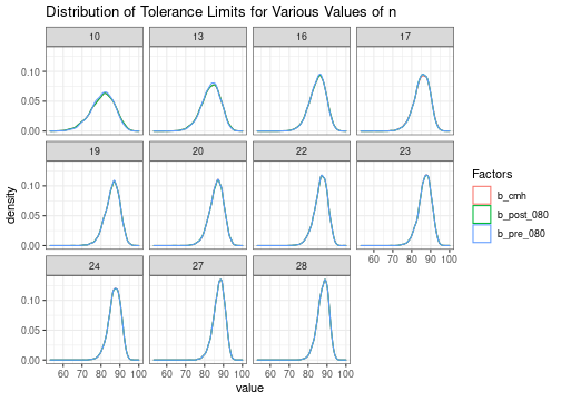
For all samples sizes, the distribution of tolerance limits is actually very similar between all three sets of factors.
The true population quantile can be calculated as follows:
x_p_normal <- qnorm(0.9, mu_normal, sd_normal, lower.tail = FALSE)
x_p_normal
#> [1] 92.31069
The proportion of calculated tolerance limit values that are below the population quantile can be calculated as follows. We see that the in all cases the tolerance limits are all conservative, and also that each set of factors produce similar levels of conservatism.
sim_normal %>%
  mutate(below_pre_080 = b_pre_080 < x_p_normal,
         below_post_080 = b_post_080 < x_p_normal,
         below_cmh = b_cmh < x_p_normal) %>%
  group_by(n) %>%
  summarise(
    prop_below_pre_080 = sum(below_pre_080) / n(),
    prop_below_post_080 = sum(below_post_080) / n(),
    prop_below_cmh = sum(below_cmh) / n()
  )
#> # A tibble: 11 × 4
#>        n prop_below_pre_080 prop_below_post_080 prop_below_cmh
#>    <dbl>              <dbl>               <dbl>          <dbl>
#>  1    10              0.984               0.980          0.980
#>  2    13              0.979               0.975          0.975
#>  3    16              0.969               0.967          0.967
#>  4    17              0.973               0.973          0.971
#>  5    19              0.962               0.961          0.961
#>  6    20              0.964               0.962          0.964
#>  7    22              0.961               0.960          0.960
#>  8    23              0.960               0.959          0.960
#>  9    24              0.962               0.961          0.962
#> 10    27              0.954               0.953          0.954
#> 11    28              0.952               0.952          0.952
Simulation with Weibull Data
Next, we’ll do a similar simulation using data drawn from a Weibull distribution. Again, we’ll generate 10,000 samples for each sample size.
shape_weibull <- 60
scale_weibull <- 100

set.seed(234568)  # make this reproducible

sim_weibull <- pmap_dfr(factor_diff, function(n, j_pre_080, z_pre_080,
                                              j_post_080, z_post_080,
                                              j_cmh, z_cmh) {
  map_dfr(1:10000, function(i_sim) {
    x <- sort(rweibull(n, shape_weibull, scale_weibull))
    tibble(
      n = n,
      b_pre_080 = tolerance_limit(x, j_pre_080, z_pre_080),
      b_post_080 = tolerance_limit(x, j_post_080, z_post_080),
      b_cmh = tolerance_limit(x, j_cmh, z_cmh),
      x = list(x)
    )
  }
  )
})
sim_weibull
#> # A tibble: 110,000 × 5
#>        n b_pre_080 b_post_080 b_cmh x
#>    <dbl>     <dbl>      <dbl> <dbl> <list>
#>  1    10      95.3       95.1  95.1 <dbl [10]>
#>  2    10      88.5       88.3  88.3 <dbl [10]>
#>  3    10      89.7       89.3  89.3 <dbl [10]>
#>  4    10      94.7       94.4  94.4 <dbl [10]>
#>  5    10      96.9       96.9  96.9 <dbl [10]>
#>  6    10      93.6       93.2  93.2 <dbl [10]>
#>  7    10      86.1       85.5  85.5 <dbl [10]>
#>  8    10      91.9       91.9  91.9 <dbl [10]>
#>  9    10      93.7       93.4  93.4 <dbl [10]>
#> 10    10      90.9       90.4  90.4 <dbl [10]>
#> # … with 109,990 more rows
The distribution of the tolerance limits for each sample size is as follows. Once again, we see that the distribution of tolerance limits is nearly identical when each of the three sets of factors are used.
sim_weibull %>%
  pivot_longer(cols = b_pre_080:b_cmh, names_to = "Factors") %>%
  ggplot(aes(x = value, color = Factors)) +
  geom_density() +
  facet_wrap(n ~ .) +
  theme_bw() +
  ggtitle("Distribution of Tolerance Limits for Various Values of n")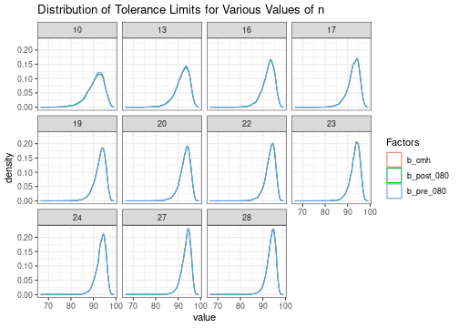
The true population quantile can be calculated as follows:
x_p_weibull <- qweibull(0.9, shape_weibull, scale_weibull, lower.tail = FALSE)
x_p_weibull
#> [1] 96.31885
The proportion of calculated tolerance limit values that are below the population quantile can be calculated as follows. We see that the in all roughly 95% or more of the tolerance limits calculated for each sample is below the population quantile. We also see very similar proportions for each of the three sets of factors considered.
sim_weibull %>%
  mutate(below_pre_080 = b_pre_080 < x_p_weibull,
         below_post_080 = b_post_080 < x_p_weibull,
         below_cmh = b_cmh < x_p_weibull) %>%
  group_by(n) %>%
  summarise(
    prop_below_pre_080 = sum(below_pre_080) / n(),
    prop_below_post_080 = sum(below_post_080) / n(),
    prop_below_cmh = sum(below_cmh) / n()
  )
#> # A tibble: 11 × 4
#>        n prop_below_pre_080 prop_below_post_080 prop_below_cmh
#>    <dbl>              <dbl>               <dbl>          <dbl>
#>  1    10              0.97                0.965          0.965
#>  2    13              0.966               0.964          0.964
#>  3    16              0.959               0.959          0.959
#>  4    17              0.961               0.961          0.96
#>  5    19              0.957               0.956          0.956
#>  6    20              0.955               0.954          0.955
#>  7    22              0.953               0.952          0.952
#>  8    23              0.950               0.950          0.950
#>  9    24              0.953               0.953          0.953
#> 10    27              0.952               0.951          0.951
#> 11    28              0.950               0.950          0.950
Conclusion
The values of
and
computed by the kh_Ext_z_j_opt function differs for certain
samples sizes
()
before and after version 0.8.0. Furthermore, for certain sample sizes,
these values differ from those published in CMH-17-1G. The simulation
study presented in this vignette shows that the tolerance limit (Basis
value) might differ for any individual sample based on which set of
and
are used. However, each set of factors produces tolerance limit factors
that are either correct or conservative. These three methods have very
similar performance, and tolerance limits produced with any of these
three methods are equally valid.
Session Info
This vignette is computed in advance. A system with the following configuration was used:
sessionInfo()
#> R version 4.1.1 (2021-08-10)
#> Platform: x86_64-pc-linux-gnu (64-bit)
#> Running under: Ubuntu 20.04.3 LTS
#>
#> Matrix products: default
#> BLAS:   /usr/lib/x86_64-linux-gnu/blas/libblas.so.3.9.0
#> LAPACK: /usr/lib/x86_64-linux-gnu/lapack/liblapack.so.3.9.0
#>
#> locale:
#>  [1] LC_CTYPE=en_CA.UTF-8       LC_NUMERIC=C               LC_TIME=en_CA.UTF-8        LC_COLLATE=en_CA.UTF-8
#>  [5] LC_MONETARY=en_CA.UTF-8    LC_MESSAGES=en_CA.UTF-8    LC_PAPER=en_CA.UTF-8       LC_NAME=C
#>  [9] LC_ADDRESS=C               LC_TELEPHONE=C             LC_MEASUREMENT=en_CA.UTF-8 LC_IDENTIFICATION=C
#>
#> attached base packages:
#> [1] stats     graphics  grDevices utils     datasets  methods   base
#>
#> other attached packages:
#> [1] tidyr_1.1.4   purrr_0.3.4   ggplot2_3.3.5 dplyr_1.0.7
#>
#> loaded via a namespace (and not attached):
#>  [1] tidyselect_1.1.1  xfun_0.26         remotes_2.4.0     colorspace_2.0-2  vctrs_0.3.8       generics_0.1.0
#>  [7] testthat_3.0.4    htmltools_0.5.2   usethis_2.0.1     yaml_2.2.1        utf8_1.2.2        rlang_0.4.11.9001
#> [13] pkgbuild_1.2.0    pillar_1.6.3      glue_1.4.2        withr_2.4.2       DBI_1.1.1         waldo_0.3.1
#> [19] cmstatr_0.9.0     sessioninfo_1.1.1 lifecycle_1.0.1   stringr_1.4.0     munsell_0.5.0     gtable_0.3.0
#> [25] devtools_2.4.2    memoise_2.0.0     evaluate_0.14     labeling_0.4.2    knitr_1.35        callr_3.7.0
#> [31] fastmap_1.1.0     ps_1.6.0          curl_4.3.1        fansi_0.5.0       highr_0.9         scales_1.1.1
#> [37] kSamples_1.2-9    cachem_1.0.6      desc_1.4.0        pkgload_1.2.2     farver_2.1.0      fs_1.5.0
#> [43] digest_0.6.28     stringi_1.7.4     processx_3.5.2    SuppDists_1.1-9.5 rprojroot_2.0.2   grid_4.1.1
#> [49] cli_3.0.1         tools_4.1.1       magrittr_2.0.1    tibble_3.1.4      crayon_1.4.1      pkgconfig_2.0.3
#> [55] MASS_7.3-54       ellipsis_0.3.2    prettyunits_1.1.1 assertthat_0.2.1  rmarkdown_2.11    rstudioapi_0.13
#> [61] R6_2.5.1          compiler_4.1.1